This article was originally published at ARM's website. It is reprinted here with the permission of ARM.
The Fast Fourier Transformation (FFT) is a powerful tool in signal and image processing. One very valuable optimization technique for this type of algorithm is vectorization. This article discusses the motivation, vectorization techniques and performance of the FFT on ARM Mali GPUs. For large 1D FFT transforms (greater than 65536 samples), performance improvements over 7x are observed.
Background
A few months ago I was involved in a mission to optimize an image-processing application. The application had multiple 2D convolution operations using large-radii blurring filters. Image convolutions map well to the GPU since they are usually separable and can be vectorized effectively on Mali hardware. However, with a growing filter size, they eventually hit a brick wall imposed by computational complexity theory.
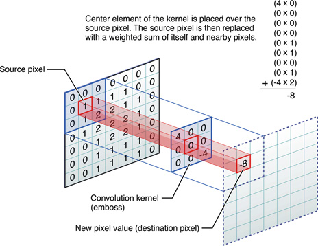
An illustration of a 2D convolution (Source: http://www.westworld.be/page/2/).
In the figure above, an input image is convolved with a 3×3 filter. For the input pixel, there will be about 9 multiplications and 8 additions required to produce the corresponding output. When estimating the time complexity of this 2D convolution, the multiplication and addition operations are assumed as a constant time. Therefore, the time complexity is approximately O(n2), although when the filter size grows, the number of operations per pixel increases and the constant time assumption can no longer hold. With a non-separable filter, the time complexity quickly approaches O(n4) as the filter size becomes comparable to the image size.
In the era of ever increasing digital image resolutions, a O(n4) time is simply not good enough for modern applications. This is where the FFT may offer an alternative computing route. With the FFT, convolution operations can be carried out in the frequency domain. The FFT forward and inverse transformation each needs O(n2 log n) time and has a clear advantage over time/spatial direct convolution which requires O(n4).
The next section assumes a basic understanding of the FFT. A brief introduction to the algorithm can be found here: http://www.cmlab.csie.ntu.edu.tw/cml/dsp/training/coding/transform/fft.html
FFT Vectorization on Mali GPUs
For simplicity, a 1D FFT vectorized implementation will be discussed here. Multi-dimensional FFTs are separable operations, thus the 1D FFT can easily be extended to accommodate higher-dimension transforms. The information flow of the FFT is best represented graphically by the classic butterfly diagram:
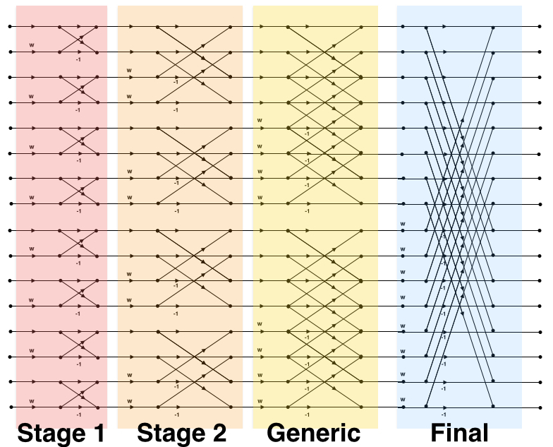
16-point Decimation in Frequency (DIF) butterfly diagram.
The transformation is broken into 4 individual OpenCL kernels: 2-point, 4-point, generic and final transformations. The generic and final kernels are capable of varying in size. The generic kernel handles transformations from 8-point to half of the full transformation. The final kernel completes the transformation by computing the full-size butterfly.
The FFT operates within the complex domain. The input data is sorted into a floating-point buffer of real and imaginary pairs:
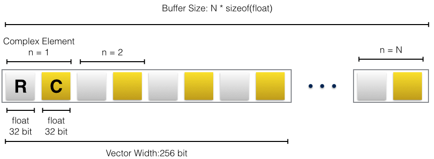
The structure of the input and output buffer. A complex number consists of two floating-point values. The vector width is also shown.
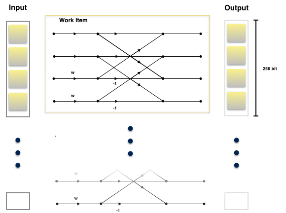
The first stage of the decimation in time (DIT) FFT algorithm is a 2-point discrete Fourier transform (DFT). The corresponding kernel consists of two butterflies. Each of these two butterflies operate on two complex elements as shown:
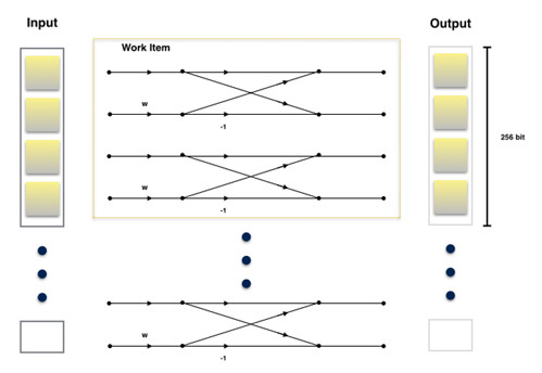
An illustration of the first stage kernel. A yellow-grey shaded square represents a single complex number. The yellow outline encloses the butterflies evaluated by a single work item. The same operation is applied to cover all samples.
Each work item has a throughput of 4 complex numbers, 256 bits. This aligns well with the vector width.
In the second stage, the butterflies have a size of 4 elements. Similar to the first kernel, the second kernel has a throughput of 4 complex number, aligning with the vector width. The main distinctions are in the twiddles and the butterfly network:
The illustration for the second stage kernel: a single 4-point butterfly.
The generic stage is slightly more involved. In general, we would like to:
- Re-use the twiddle factors
- Keep the data aligned to the vector width
- Maintain a reasonable register usage
- Maintain a good ratio between arithmetic and data access operations
These requirements help to improve the efficiency of memory access and ALU usage. They also help to ensure that optimal numbers of work items can be dispatched at a time. With these requirements in mind, each work item for this kernel is responsible for 4 complex numbers for 4 butterflies. The kernel essentially operates on 4 partial butterflies and has a total throughput of:
4 complex number * 2 float * sizeof(float) * 4 partial butterflies = 1024 bit per work item
This is illustrated in the following graph:
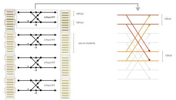
The graph above represents the 8-point butterfly case for the generic kernel. The left side of the diagram shows 4 butterflies, which associate with a work item. The red boxes on the left diagram highlight the complex elements being evaluated by the work item. The drawing on the right is a close-up view of a butterfly. The red and orange lines highlight the relevant information flow of the butterfly.
Instead of evaluating a single butterfly at a time, the kernel works on portions of multiple butterflies. This essentially allows the same twiddle factors to be re-used across the butterflies. For an 8-point transform as shown in the graph above, the butterfly would be distributed across 4 work items. The kernel is parameterizable from 8-point to N/2 point transform where N is the total length of the original input.
For the final stage, only a single butterfly of size N exists; twiddle factor sharing is not possible. Therefore, the final stage is just vectorized butterfly network that is parameterized to a size of N.
Performance
The performance of the 1D FFT implementation described in the last section is compared to a reference CPU implementation. In the graph below, the relative performance speed up is shown from 26 to 217 samples. Please note that the x-axis is on a log metric scale:
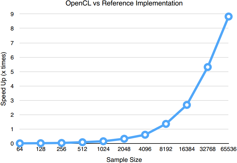
GPU FFT performance gain over the reference implementation.
We have noticed in our experiments that FFT algorithm performance tends to improve significantly on the GPU between about 4096 and 8192 samples The speed up continues to improve as the sample sizes grows. The performance gain essentially offsets the setup cost of OpenCL with large samples. This trend would be more prominent in higher dimension transformations.
Summary
The FFT is a valuable tool in digital signal and image processing. The 1D FFT implementation presented can be extended to higher dimension transformations. Applications such as computational photography, computer vision and image compression should benefit from this. What is more interesting is that the algorithm scales well on GPUs. The performance will further improve with more optimization and future support of half-float.
By Neil Tan
Software Engineer, ARM