This article was originally published at ARM's website. It is reprinted here with the permission of ARM. For more information, please see ARM's developer site, which includes a variety of GPU Compute, OpenCL and RenderScript tutorials.
In this third and last part of this blog series we are going to extend the mixed-radix FFT OpenCL™ implementation to two dimensions and explain how to perform optimisations to achieve good performance on Mobile ARM® Mali™ GPUs. After a short introduction why two-dimensional Fourier transform is an important and powerful tool the first section covers the mathematical background that lets us reuse the existing one-dimensional approach to build the two-dimensional implementation. Afterwards all the steps are described individually and the details are explained. Finally, at the end of each section we show the performance improvements achieved.
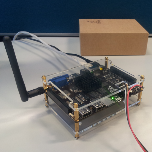
So far only the one-dimensional Fourier transform has been considered to explain the mathematical background and basic optimisations. However, in the field of image processing the two-dimensional variant is much more popular. For instance, a simple high-pass filter can be realised in the frequency domain after the image have been transformed by a two-dimensional Fourier transform. The resulting image could be used to implement an edge detection algorithm.
|
|
|
|
|
|
Original image (spatial domain) |
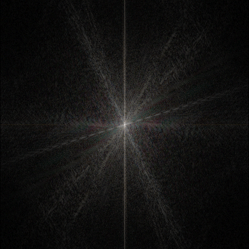
Original image (frequency domain) |
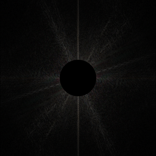
Removed high frequencies |
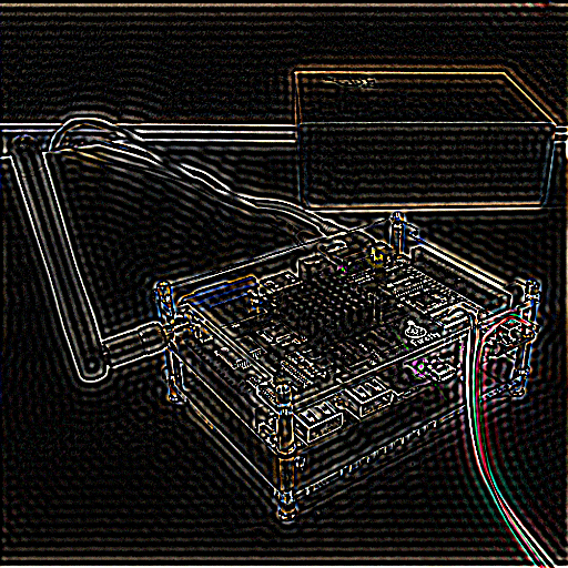
Filtered image (spatial domain) |
|
High-pass filter via Fourier transform |
|||
In general the Fourier transformation can be used to make the convolution operations which are used in many image processing applications more efficient. In particular when the kernel size is big the improvements in terms of the number of operations that have to be executed are significant. In the spatial domain a two-dimensional convolution requires a quadratic number of multiplications and a linear number of additions in the order of the size of the convolution kernel for every element of the image. Therefore the resulting complexity is O(MNmn). In contrast, in the frequency domain the convolution corresponds to a pointwise multiplication of the transformed kernel and image which reduces the complexity for the convolution to O(MN). Nevertheless, since the Fourier transform has to be additionally computed it is not always beneficial to perform the convolution in the frequency domain.
Background
Due to its separability the two-dimensional Fourier transformation can be expressed as two consecutive one-dimensional transformations. The mathematical principles are no different from those explained in the first part of this blog series which means that this background section will be rather short. It just shows briefly how the general form of the two-dimensional discrete Fourier transform can be split into its one-dimensional parts.
The two dimensional DFT can be expressed in the form
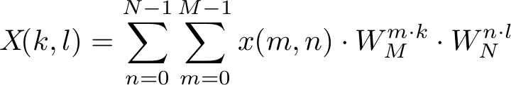
where the trigonometric constant coefficients are defined as
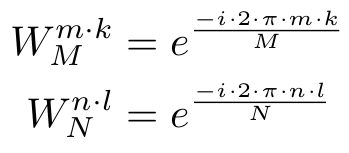
The coordinates k and l of the frequency domain are in the range

Since each of the trigonometric constant coefficients depends only on one of the summation indices the inner sum can be extracted and defined as
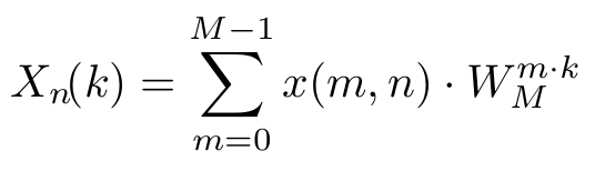
which is equal to the definition which was previously used to express the one-dimensional DFT. Only the parameter n had to be added to select the correct value in the two-dimensional input space.
If the newly defined one-dimensional transform is inserted into the original expression for the two-dimensional DFT it is easy to see from the following equation that just another one-dimensional transform is calculated
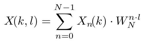
Because of the commutativity of the operations either of the sums can be extracted. Therefore it does not matter over which dimension the first one-dimensional transform is calculated.
Implementations
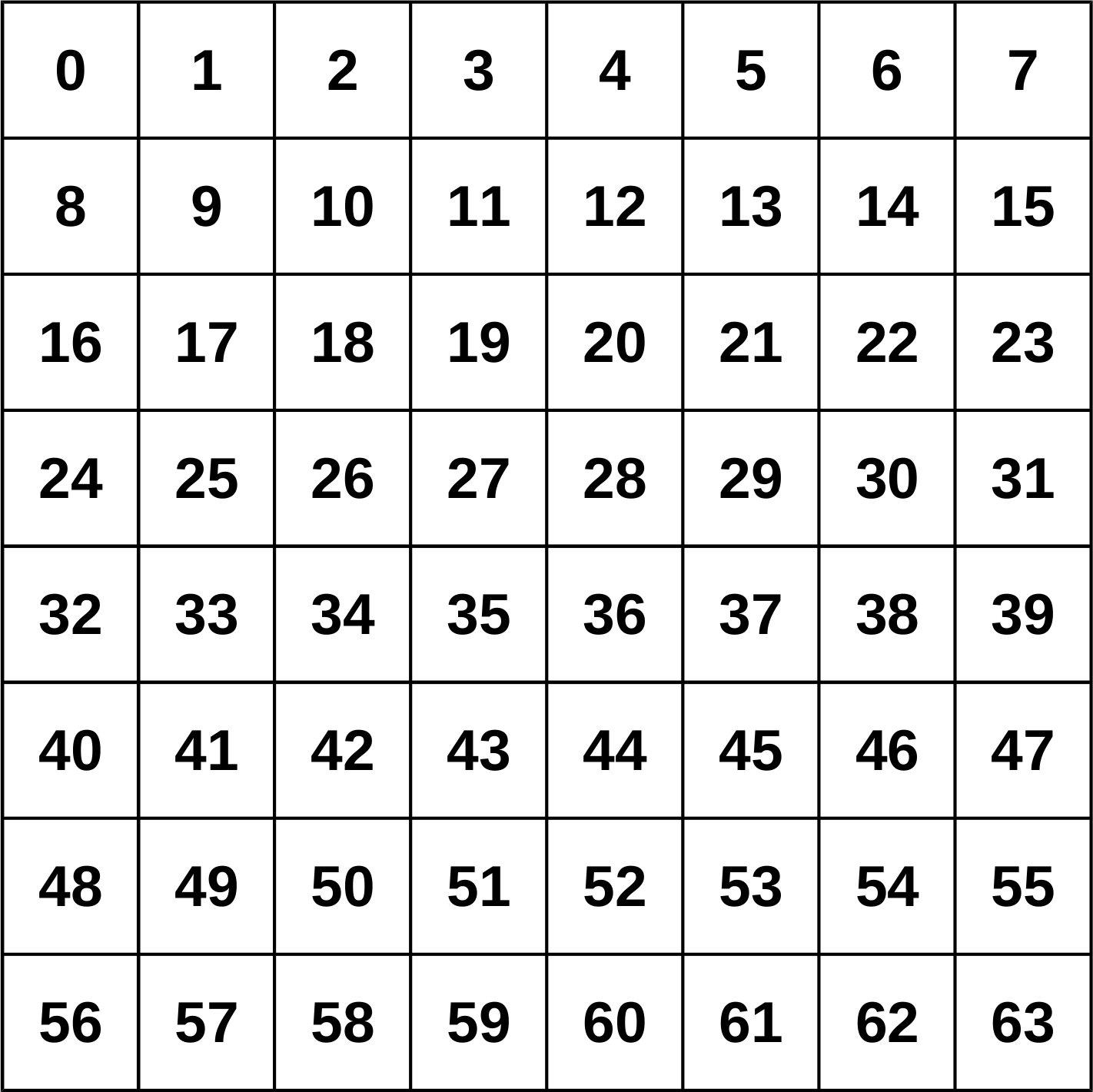
In the background section the separability of the two-dimensional Fourier transform has been used to represent the two-dimensional as two consecutive one-dimensional transforms, one along each dimension. The row-column algorithm is based on this mathematical fact and is used for this implementation. In this algorithm first a one-dimensional FFT is computed individually for every row of the two-dimensional input data. Afterwards a second one-dimensional FFT is performed for every column. But, instead of having two different functions to compute the FFT for the rows and columns, the same function is used and the input data is transposed between and after the two one-dimensional FFTs. This makes sense because the data layout is assumed to be row-major. Thus the most efficient way in terms of cache locality is to load data along the rows.
|
|
|
|
|
|
|
|
|
|
|
|
|
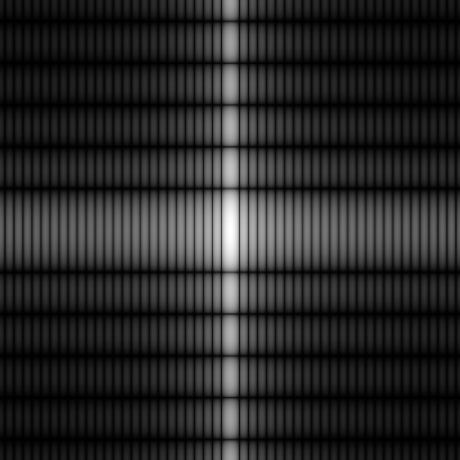
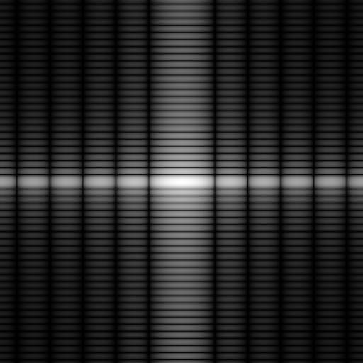
Original image |
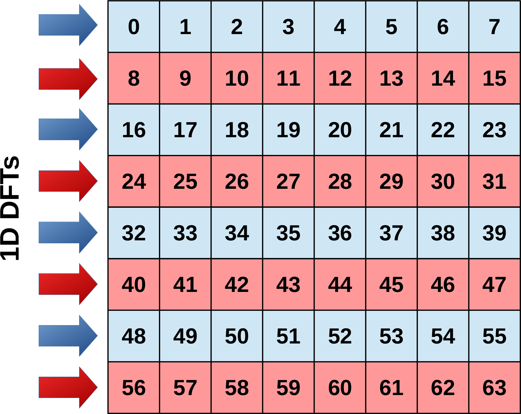
Separate 1D FFTs along the rows (first dimension) |
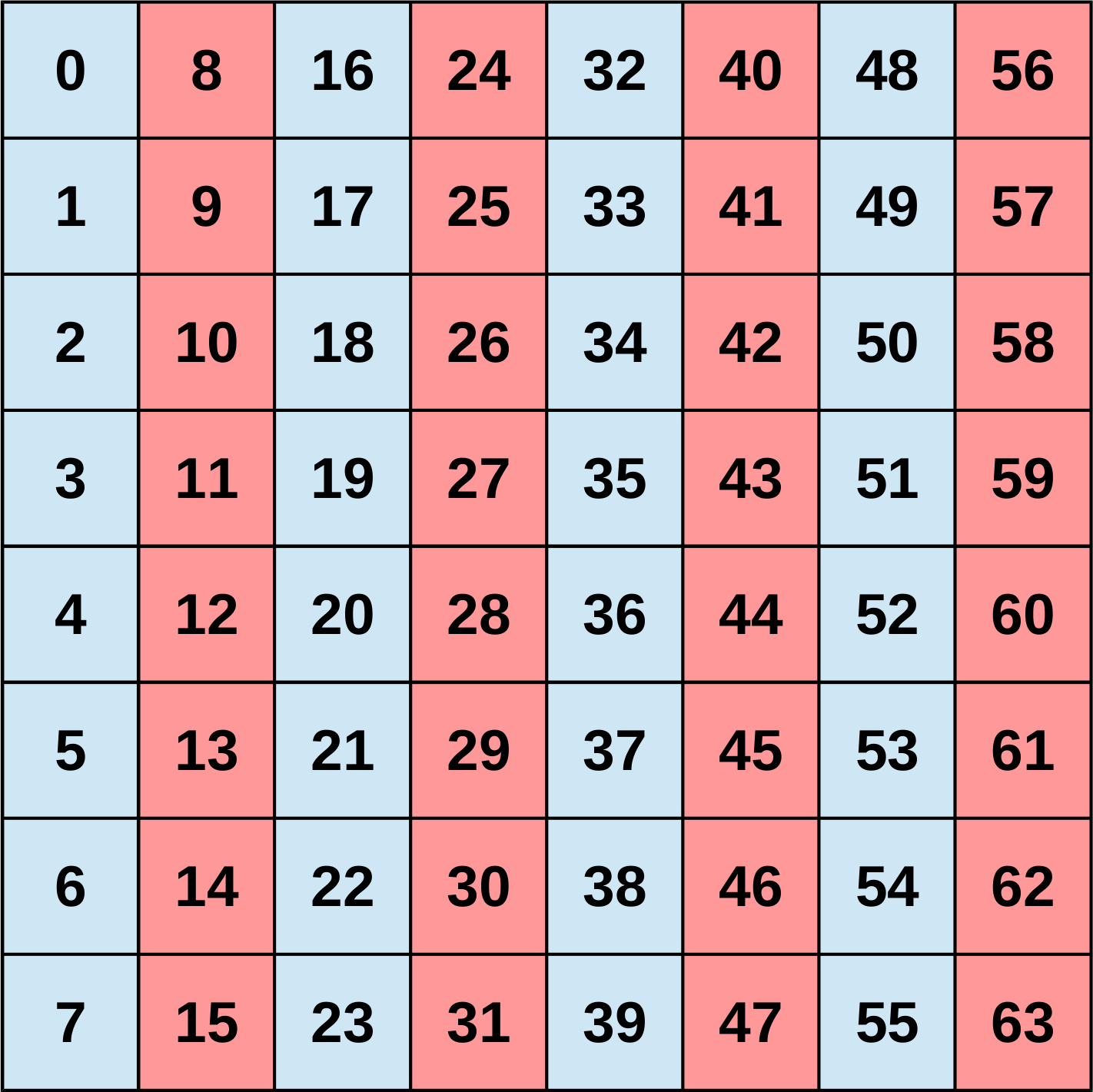
Transpose intermediate image |
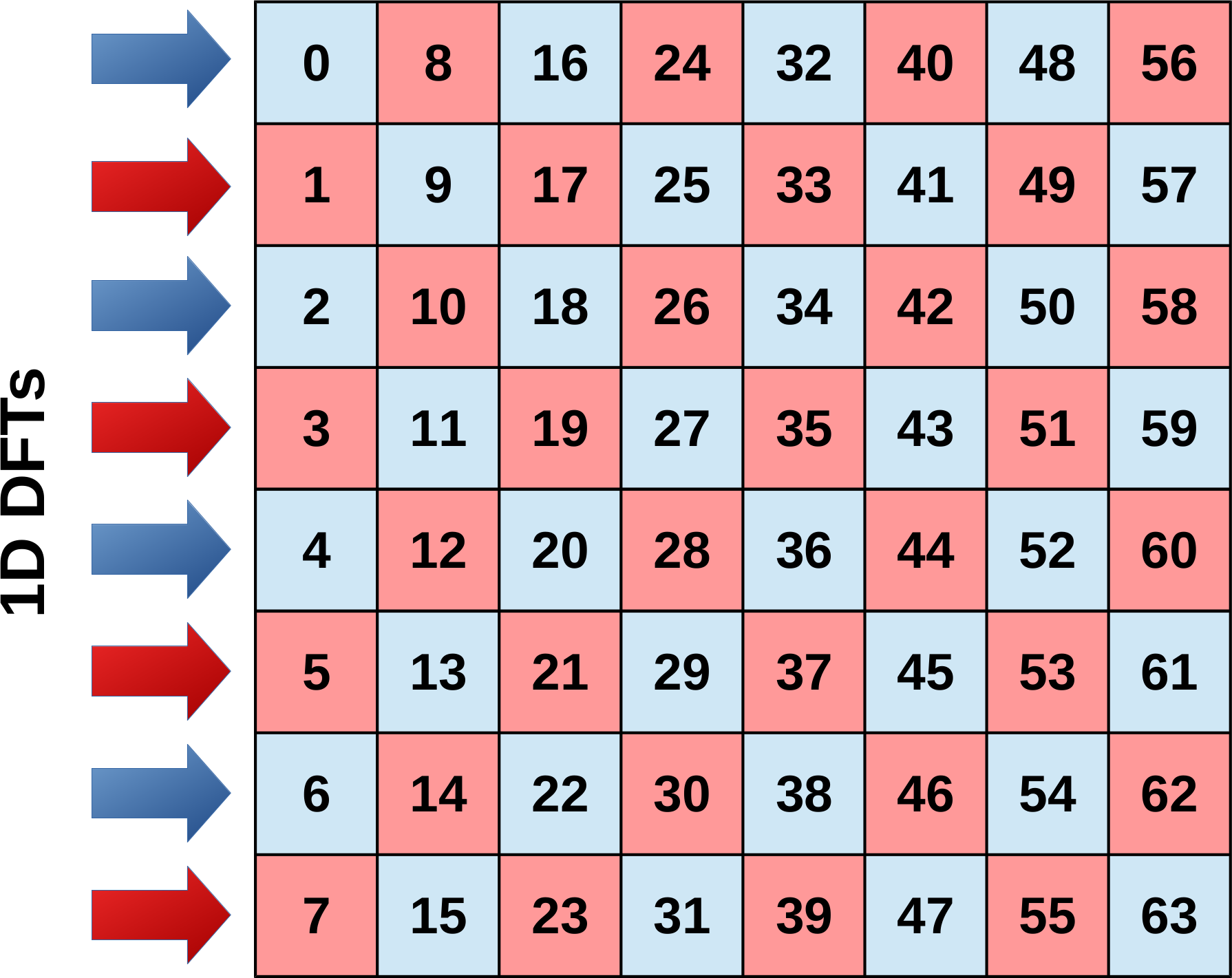
Separate 1D FFTs along the rows (second dimension) |
Transpose final image |
|
Schematics and example of the row-column algorithm |
||||
Naive row-column algorithm
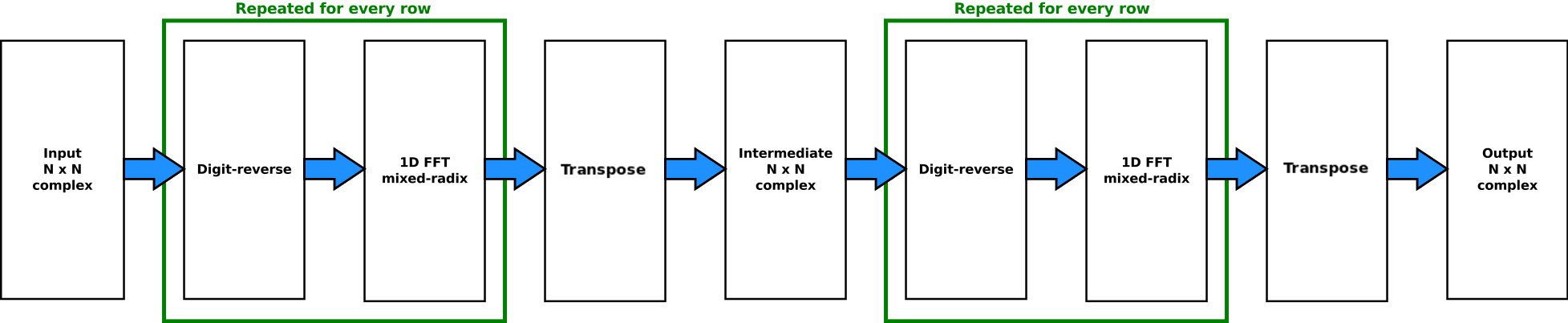
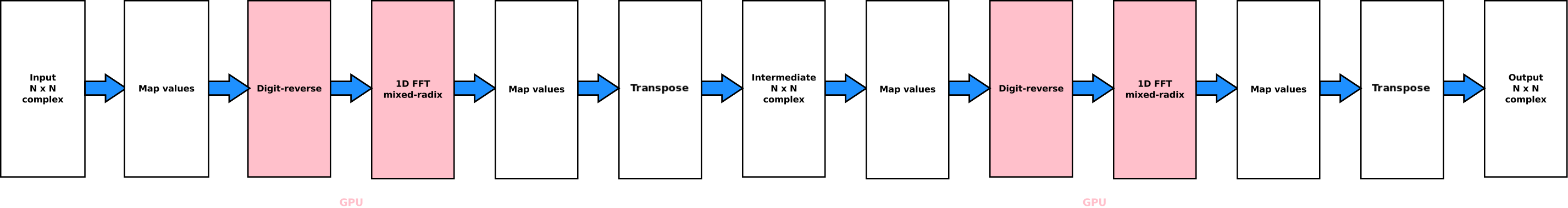
The naive implementation directly realises the principle of the row-column algorithm and the execution of the 2D FFT is therefore straightforward. The following diagram provides a first overview over the different stages of the 2D FFT and the pseudo code demonstrates the idea of a naive implementation.
Pseudo code
// Run the 1D FFT along the rows of the input buffer
// The result is stored to a temporary buffer
fft_mixed_radix_2d_run_1d_part(input, tmp);
// Transpose the intermediate buffer in-place
transpose_complex_list(tmp);
// Run the 1D FFT along the rows of the (transposed) intermediate buffer
// Corresponds to the columns of the original buffer
// The result is stored to the output buffer
fft_mixed_radix_2d_run_1d_part(tmp, output);
// Transpose the output buffer in-place
transpose_complex_list(output);
The function to compute the 1D FFT is conceptually the same that has been used in the previous parts of this blog series except that it has to loop over all rows of the source image. As a reminder: The chosen variant of the mixed radix FFT requires the input values to be in digit-reversed order to compute the output values in linear order. Therefore the input values have to be shuffled before the actual FFT can be computed. The reordering is repeated for all rows of the matrix. Similarly the computation of the 1D FFT is repeated for all rows independently of each other.
/**
* @brief Computes a 1D FFT for each row of the the input
*
* @param[in] input The input matrix
* @param[out] output The output matrix
*/
fft_mixed_radix_2d_run_1d_part(input, output)
{
// Iterate over all row of the input matrix
for(row_in in input and row_out in output)
{
// Perform digit-reverse reordering
rev_row = digit_reverse(row_in);
// Calculate mixed radix 1D FFT using the reversed row
row_out = …
}
}
Naive implementation based on OpenCL mixed-radix kernels
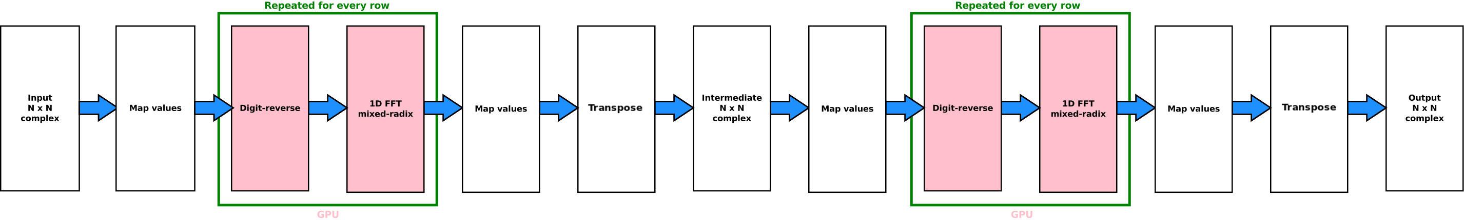
This optimisation does not introduce anything terribly new compared to the optimisation of the one-dimensional Fourier transform. The first speedup over the CPU implementation can be achieved by running the computation of the actual FFT on the GPU. For this purpose the buffer with the input values has to be mapped to a CLBuffer. Afterwards the reordering to digit-reversed order is performed on the GPU. The rows of the matrix can be reordered independently such that a one-dimensional kernel is enqueued for each one. The reordering is followed by the first one-dimensional part of the FFT which is now also computed on the GPU. Once the computation has finished the buffers are mapped again to perform the matrix transpose between the two stages of the FFT on the CPU and out-of-place. Subsequently, the rows are another time reordered and the second one-dimensional FFT is computed. Finally the results of the second stage are again transposed to restore the original data layout and copied over to the output buffer.
A loop is used to enqueue separate and independent one-dimensional kernels for each row of the input data. The kernels take the offset of the row within the linearised data representation as argument buf_offset_float.
Because each complex element of the buffer is represented through two floating point numbers (real and imaginary part) the row offset has to be doubled to get the actual offset within the buffer.
// Digit reverse stage
// Uses a 1D NDRange within the loop to process all rows of the buffer
const size_t digit_rev_gws[] = {N};
for(uint row = 0; row < N; ++row)
{
uint buf_offset_float = row * N * 2;
clSetKernelArg(digit_reverse_kernel, 0, sizeof(cl_mem), input_buf);
clSetKernelArg(digit_reverse_kernel, 1, sizeof(cl_mem), digit_reversed_buf);
clSetKernelArg(digit_reverse_kernel, 2, sizeof(cl_mem), idx_bit_reverse_buff);
clSetKernelArg(digit_reverse_kernel, 3, sizeof(cl_uint), &buf_offset_float);
clEnqueueNDRangeKernel(queue, digit_reverse_kernel, 1, NULL, digit_rev_gws, NULL, 0, NULL, NULL);
}
// Perform 2D FFT
// Uses 1D NDRange within the loop to process all rows of the buffer
for(uint row = 0; row < N; ++row)
{
uint buf_stride_float = N * 2;
uint Nx = 1;
uint Ny = radix_stage[0];
// First stage
const size_t first_stage_gws[] = {N / Ny};
clSetKernelArg(first_stage_radix_kernel, 0, sizeof(cl_mem), digit_reversed_buf);
clSetKernelArg(first_stage_radix_kernel, 1, sizeof(cl_uint), &buf_stride_float);
clEnqueueNDRangeKernel(queue, first_stage_radix_kernel, 1, NULL, first_stage_gws, NULL, 0, NULL, NULL);
// Update Nx
Nx *= Ny;
// Following stages
for(uint s = 1; s < n_stages; ++s)
{
// …
}
}
/**
* @brief Computes the first stage of a radix-2 DFT.
*
* @param[in, out] input The complex array.
* @param[in] offset The offset of the current row in the array.
*/
kernel void radix_2_first_stage(global float* input, const uint offset)
{
// Each work-item computes a single radix-2
uint idx = get_global_id(0) * 4;
// Load two complex input values
// The row_offset needs to be multiplied by two because complex numbers
// are represented through two float values
float4 in = vload4(0, input + offset + idx);
// Compute DFT N = 2
DFT_2(in.s01, in.s23);
// Store two complex output values
// The row_offset needs to be multiplied by two because complex numbers
// are represented through two float values
vstore4(in, 0, input + offset + idx);
}
Replacing loops with two-dimensional kernels
In the first, naive GPU implementation separate one-dimensional kernels are enqueued for every row of the matrix. The performance can be significantly increased by using kernels with a two-dimensional NDRange instead of loops. The second dimension is then used as a replacement for the row offset within the linearised data structure which was previously incremented in the loop. In addition to the offset in the second dimension the offset in the buffer depends also on the size of the matrix which is passed as parameter N. Again the offset needs to be multiplied by two to account for the two part complex numbers.
First of all this change reduces the number of kernels and therefore the overhead of enqueuing and dispatching them. Moreover it increases the number of work items which can be executed in parallel since in principle work items from all rows can be executed in parallel. Before, the kernels had to be executed one after the other and thus there was only a comparably small number of work items at any point in time. This reduces the GPU's utilisation, particularly for small matrices.
// Digit reverse stage
// Uses a 2D NDRange to process all rows of the buffer
const size_t digit_rev_gws[] = {N, N};
clSetKernelArg(digit_reverse_kernel, 0, sizeof(cl_mem), input_buf);
clSetKernelArg(digit_reverse_kernel, 1, sizeof(cl_mem), digit_reversed_buf);
clSetKernelArg(digit_reverse_kernel, 2, sizeof(cl_mem), idx_bit_reverse_buf);
clSetKernelArg(digit_reverse_kernel, 3, sizeof(cl_uint), &N);
clEnqueueNDRangeKernel(queue, digit_reverse_kernel, 2, NULL, digit_rev_gws, NULL, 0, NULL, NULL);
uint buf_stride_float = N * 2;
// First stage
// Uses a 2D NDRange to process all rows of the buffer
uint Nx = 1;
uint Ny = radix_stage[0];
const size_t first_stage_gws[] = {N / Ny, N};
clSetKernelArg(first_stage_radix_kernel, 0, sizeof(cl_mem), digit_reversed_buf);
clSetKernelArg(first_stage_radix_kernel, 1, sizeof(cl_uint), &buf_stride_float);
clEnqueueNDRangeKernel(queue, first_stage_radix_kernel, 2, NULL, first_stage_gws, NULL, 0, NULL, NULL);
// Update Nx
Nx *= Ny;
// Following stages
for(uint s = 1; s < n_stages; ++s)
{
// …
}
/**
* @brief Computes the first stage of a radix-2 DFT.
*
* @param[in, out] input The complex array.
* @param[in] buf_stride_float The number of floats per row in the array.
*/
kernel void radix_2_first_stage(global float* input, const uint buf_stride_float)
{
// Each work-item computes a single radix-2
uint idx = get_global_id(0) * 4;
// Compute the offset into the buffer for the current row
// Needs to be multiplied by two because complex numbers
// are represented through two float values
const uint offset = get_global_id(1) * buf_stride_float; // <– Previously computed in the host code
// Load two complex input values
float4 in = vload4(0, input + offset + idx);
// Compute DFT N = 2
DFT_2(in.s01, in.s23);
// Store two complex output values
vstore4(in, 0, input + offset + idx);
}
Parallel transpose on the GPU
The next optimisation moves the transpose operation so it is also running on the GPU. If it is not performed in-place there are no dependencies between the individual elements at all and the transpose can be fully executed in parallel. For in-place algorithms at least two elements have to swapped in each step as otherwise information would be overwritten.
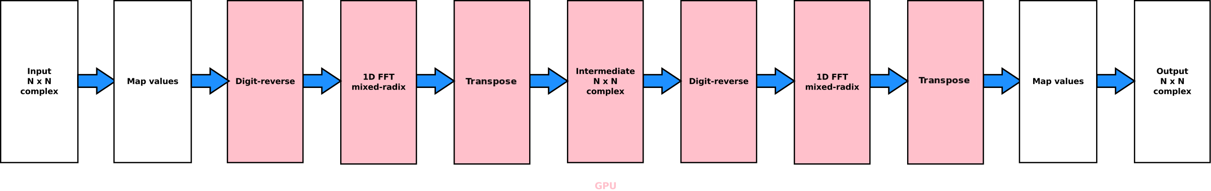
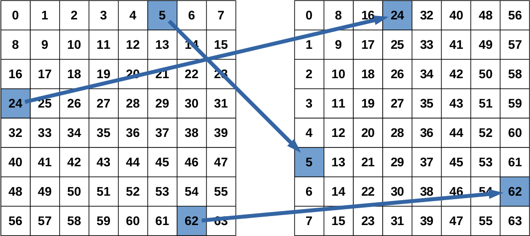
Parallel elementwise out-of-place transpose
This approach resembles the CPU variant of a naive elementwise transpose of a matrix. Each work item reads one element according to its global id from the source buffer and writes it to the corresponding transposed position in the output buffer. The global work group size is thus equal to the size of the matrix (N x N). The elements themselves consist of two floating point values which represent the real and imaginary parts of the complex values.
/**
* @brief Transposes a quadratic matrix of complex numbers stored in row major order.
*
* @param[in] input The complex input array.
* @param[out] output The complex output array.
* @param[in] buf_stride_complex The number of complex numbers per row in the array.
*/
kernel void transpose(global float2* input, global float2* output, const uint buf_stride_complex)
{
uint ix = get_global_id(0);
uint iy = get_global_id(1);
output[ix * buf_stride_complex + iy] = input[iy * buf_stride_complex + ix];
}
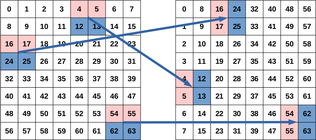
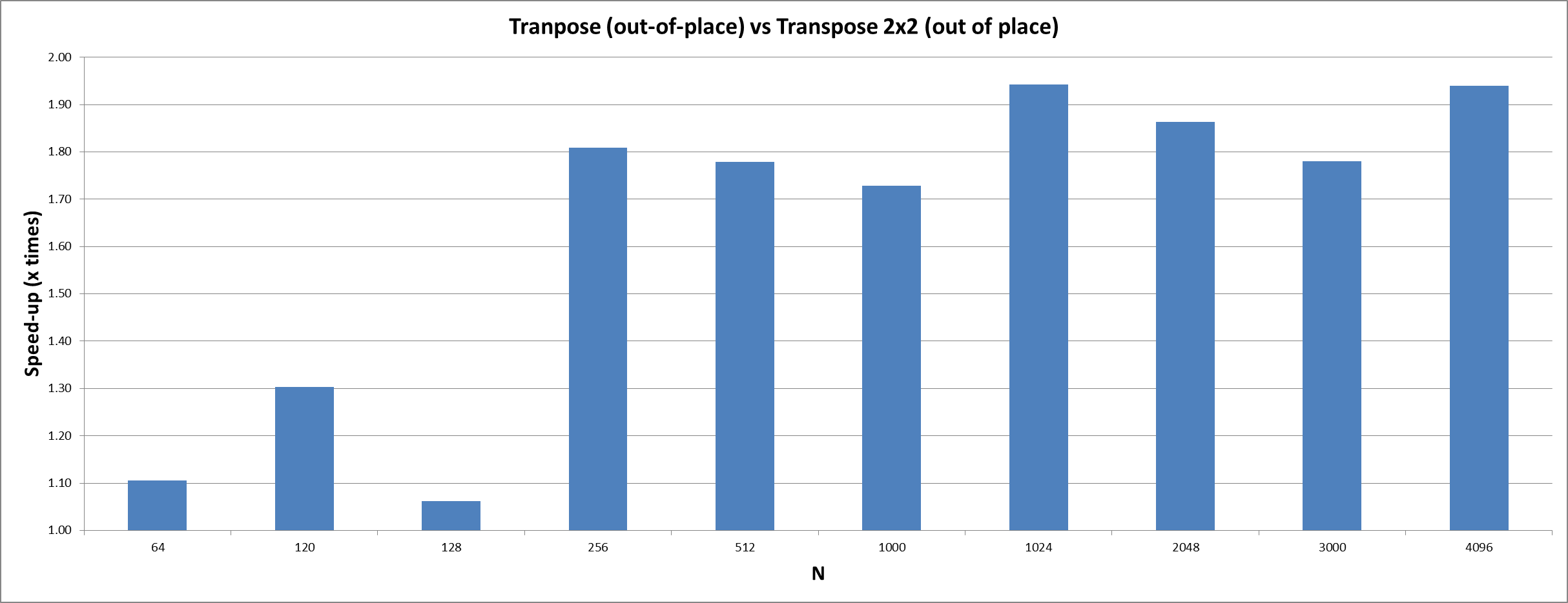
Parallel blockwise out-of-place transpose
However, this simple approach is not efficient enough to compensate for the additional driver overhead for launching kernels when performing the transpose on the GPU. To increase the performance the transpose operation has to be executed blockwise instead of elementwise. Instead of reading and writing one pixel per work item a small sub-block of the complete matrix is loaded. It is then locally transposed and written back to the corresponding position in the output matrix.
Compared to the naive transpose approach this optimisation increases the cache efficiency and the resource utilisation since each work item operates on more than one pixel. Further it helps to increase the utilisation of the GPU resources by making the kernels larger and slightly more complex. As a result the number of work items decreases which reduces the overhead of dispatching work items for executuion. The choice of two-by-two sub-blocks turned out to be optimal since the local transpose of larger sub-blocks requires more registers.
/**
* @brief Transposes a quadratic matrix of complex numbers stored in row major order.
*
* @param[in] input The complex input array.
* @param[out] output The complex output array.
* @param[in] buf_stride_float The number of floats per row in the array.
*/
kernel void transpose2x2(global float* input, global float* output, const uint buf_stride_float)
{
const uint ix = get_global_id(0);
const uint iy = get_global_id(1);
float4 tmp;
float4 u0, u1;
// Load one sub-block from two rows
u0 = vload4(ix, input + (iy * 2) * buf_stride_float);
u1 = vload4(ix, input + (iy * 2 + 1) * buf_stride_float);
// Transpose the sub-block
tmp = u0;
u0 = (float4)(tmp.s01, u1.s01);
u1 = (float4)(tmp.s23, u1.s23);
// Write the sub-block to the transposed position
vstore4(u0, iy, output + (ix * 2) * buf_stride_float);
vstore4(u1, iy, output + (ix * 2 + 1) * buf_stride_float);
}
Speedup
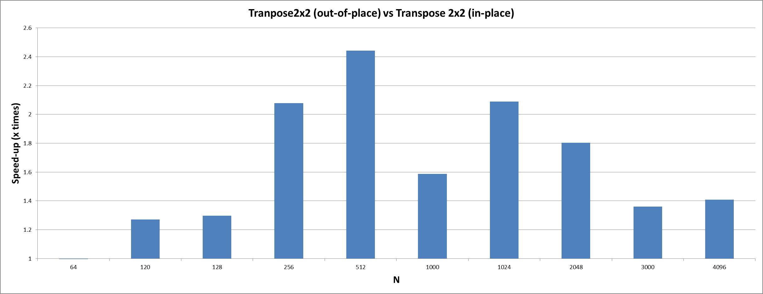
Parallel blockwise in-place transpose
Due to its nature a transpose operation can be realised by always swapping to corresponding elements or larger sub-blocks respectively. This allows us to load, transpose and store two sub-blocks per work item in order to reduce the number of work items and to achieve a better balance between arithmetic and load/store operations. As a side-effect the transpose algorithm can be changed from out-of-place to in-place such that the second buffer is no longer needed.
As a consequence of the transpose-and-swap approach it would be sufficient to have one work item for each block in the upper triangular matrix. However, if a one-dimensional kernel is enqueued with the smallest possible number of work items the transformation of the linear index into the two-dimensional index is less efficient than simply using a two-dimensional kernel and aborting the work items below the diagonal. The diagonal itself requires special treatment because the diagonal sub-blocks do not need to be exchanged with a different sub-block but only have to be transposed locally.
/**
* @brief Transposes a quadratic matrix of complex numbers stored in row major order.
*
* @param[in, out] input The complex array.
* @param[in] buf_stride_float The number of floats per row in the array.
*/
kernel void transpose2x2(global float* input, const uint buf_stride_float)
{
const uint ix = get_global_id(0);
const uint iy = get_global_id(1);
// Abort for sub-blocks below the diagonal
if(ix < iy)
{
return;
}
float4 tmp;
float4 v0, v1, u0, u1;
// Load first sub-block
u0 = vload4(ix, input + (iy * 2) * buf_stride_float);
u1 = vload4(ix, input + (iy * 2 + 1) * buf_stride_float);
// Transpose first sub-block
tmp = u0;
u0 = (float4)(tmp.s01, u1.s01);
u1 = (float4)(tmp.s23, u1.s23);
// Only process a second sub-block if the first one is not on the diagonal
if(ix != iy)
{
// Load second sub-block
v0 = vload4(iy, input + (ix * 2) * buf_stride_float);
v1 = vload4(iy, input + (ix * 2 + 1) * buf_stride_float);
// Transpose second sub-block
tmp = v0;
v0 = (float4)(tmp.s01, v1.s01);
v1 = (float4)(tmp.s23, v1.s23);
// Store second sub-block to transposed position
vstore4(v0, ix, input + (iy * 2) * buf_stride_float);
vstore4(v1, ix, input + (iy * 2 + 1) * buf_stride_float);
}
// Store first sub-block to transposed position
vstore4(u0, iy, input + (ix * 2) * buf_stride_float);
vstore4(u1, iy, input + (ix * 2 + 1) * buf_stride_float);
}
![]()
Speedup
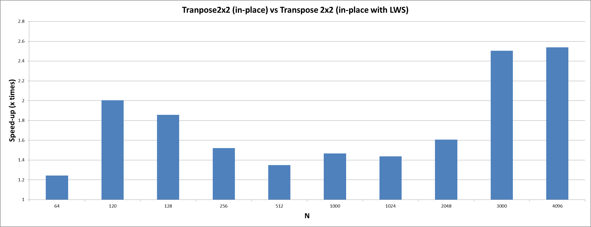
Setting local work group size
For the two-dimensional transpose kernel the automatically inferred values for the local work group size were not able to achieve good performance. It turned out to be better to set the local work group size manually to a size of 2 x 4 – or smaller if the buffer (divided by two because each work items handles a 2 x 2 sub-block) is not a multiple of 4. The best size for the local work groups always depends on the kernel and finding a good size can be hard. However, getting the sizes right can help to achieve better caching behaviour and therefore can improve runtime performance.
// Setting up constants
// For odd matrix sizes padding is necessary
// because the transpose kernel stores two complex values
const size_t padding = 2 * (N % 2);
const size_t buf_stride_float = N * 2 + padding;
const size_t buf_stride_half = buf_stride_float / 2;
clSetKernelArg(transpose_kernel, 0, sizeof(cl_mem), fft_buf);
clSetKernelArg(transpose_kernel, 1, sizeof(cl_uint), &buf_stride_float);
// Set global work group size
const size_t transpose_gws[2] = {buf_stride_half, buf_stride_half};
size_t transpose_lws[2];
size_t *transpose_lws_ptr;
// Determine the largest possible local work group size
// It has to divide the global work group size
if(buf_stride_half % 4 == 0)
{
transpose_lws[0] = 2;
transpose_lws[1] = 4;
transpose_lws_ptr = transpose_lws;
}
else if(buf_stride_half % 2 == 0)
{
transpose_lws[0] = 1;
transpose_lws[1] = 2;
transpose_lws_ptr = transpose_lws;
}
else
{
transpose_lws_ptr = NULL;
}
clEnqueueNDRangeKernel(queue, transpose_kernel, 2, NULL, transpose_gws, transpose_lws_ptr, 0, NULL, NULL);
Speedup
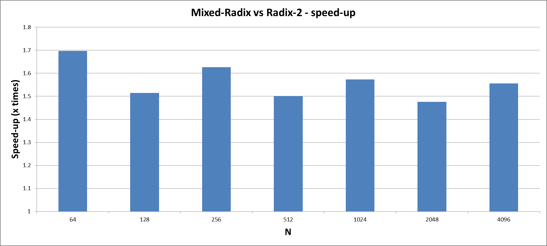
Comparison to radix-2 implementation
The following diagram visualises the benefit in terms of a shorter runtime when the mixed-radix variant is used instead of a radix-2 only implementation. Note the logarithmic scaling of the y-axis. Another advantage of a mixed-radix approach over a radix-2 only FFT is the larger number of supported sizes. For instance, FFTs for matrix sizes 120, 1000 and 3000 can not be computed with the radix-2 only approach and are therefore missing in the diagram.
Conclusion
While this pushes the row-column algorithm to its boundaries it might be possible to achieve better performance if the underlying FFT algorithm is changed. For instance, if the FFT is not computed in-place the digit-reversal could be dropped and moreover the transpose could be merged into the mixed-radix FFT kernels. However, it is difficult to predict the benefits if there are any.
Useful optimisation aspects
The following list summarises the things that have been considered to increase the performance of the 2D FFT mixed-radix algorithm on Mobile ARM® Mali™ GPUs in this article:
- Instead of enqueuing many one-dimensional kernels in a loop it is better to use one/fewer higher-dimensional kernel/s.
- The optimal size of the sub-blocks for the blocked transpose depends on the available resources. Increasing the block size has only positive effects as long as the cache is big enough and sufficient registers are available.
- Padding buffers can help to generalise kernels and can prevent branches in the control flow. For instance, the mapped buffers are padded to the next larger even size in both dimensions to eliminate edge cases during the transpose operation.
- Loads and stores are most efficient if they are performed according to the data layout because only then the cache efficiency is more optimal.
- It can be more efficient to conditionally abort superfluous work items in a 2D range directly instead of computing the two-dimensional index out of a linear index.
- Find ways to parallelize sequential code and keep work items as independent from each other as possible.
- Compute more than one pixel (or more bytes) per work item.
- Reduce the number of load/store operations by vectorising. This is especially beneficial because the GPU comprises a vector unit (SIMD).
Further reading
- http://paulbourke.net/miscellaneous/dft/
- http://fourier.eng.hmc.edu/e101/lectures/Image_Processing/node6.html
By Gian Marco Iodice
GPU Compute Software Engineer, ARM