This article was originally published at NVIDIA’s website. It is reprinted here with the permission of NVIDIA.
This article discusses how an application developer can prototype and deploy deep learning algorithms on hardware like the NVIDIA Jetson Nano Developer Kit with MATLAB. In previous posts, we explored how you can design and train deep learning networks in MATLAB and how you can generate optimized CUDA code from your deep learning algorithms.
In our experience working with deep learning engineers, we often see they run into challenges when prototyping with real hardware because they have to manually integrate their entire application code, such as interfaces with the sensors on the hardware, or integrate with the necessary toolchain to deploy and run the application on the hardware. If the algorithm does not have the expected behavior or if it does not meet the performance expectation, they have to go back to their workstation to debug the underlying cause.
This post shares how an application developer can deploy, validate and verify their MATLAB algorithms on real hardware like the NVIDIA Jetson platform by:
- Using live data from the Jetson board to improve algorithm robustness
- Using hardware-in-the-loop simulation for verification and performance profiling
- Deploying standalone applications on the Jetson board
Using NVIDIA Jetson with MATLAB
MATLAB makes it easier to prototype and deploy to NVIDIA hardware through the NVIDIA hardware support package. It provides simple APIs for interactive workflow as well as standalone execution and enables you to:
- Connect directly to the hardware from MATLAB and test your application on sensor data from the hardware
- Deploy the standalone application to the Jetson board
- Debug any issues before deploying a standalone application to the Jetson board
These workflows steps are illustrated in the figure below:
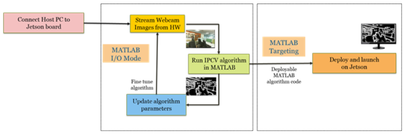
Figure 1: Illustrating the three steps of the workflow
The support package supports the NVIDIA Jetson TK1, Jetson TX1, Jetson TX2, Jetson Xavier and Jetson Nano developer kits. It also supports the NVIDIA DRIVE platform. Below is the pseudo code using these APIs to work with the NVIDIA hardware using MATLAB:
% builtin APIs to connect to Jetson hardware
hwobj= jetson(‘jetsonnano’,’username’,’password’);
% APIs to fetch sensor data and run inference in MATLAB for validation
input_img=hwobj.webcam.snapshot;
output=InferenceFunction(input_img);
% Generate code and configure it to run in hardware in loop mode
codegen(‘-config’,cfg,’InferenceFunction’,’-args’,{test_img},’-report’);
%Run the inference on the hardware and verify
output_new=InferenceFunction_pil(input_img);
compare(output, output_new);
Defect Detection Example
Let us consider an industrial automation application for defect detection from one of our customers who used GPU Coder to deploy their deep learning application to detect abnormalities in manufactured parts using a Jetson developer kit. We will consider a similar application as an example and develop a deep learning algorithm to detect defects in manufactured nuts and bolts, but this extends naturally for other application areas like predictive maintenance of industrial equipment, etc.
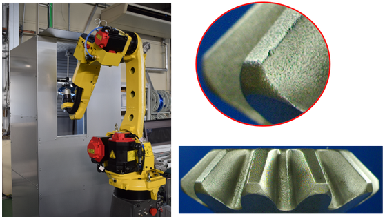
Figure 2: Automated inspection of 1.3 million bevel gear per month to detect abnormalities in Automotive parts
We recently hosted a webinar titled “Deep Learning on Jetson Using MATLAB, GPU Coder, and TensorRT” that explains how you can train a network in MATLAB and generate optimized CUDA code that leverages NVIDIA TensorRT, a deep learning inference platform, for Jetson boards. Figure 4 shows the algorithm pipeline including the pre- and post-processing steps that include typical image processing steps like identifying the region of interest, resizing the input image and finally annotating the output image.
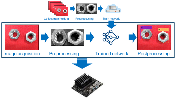
Figure 3: The algorithm pipeline
function out = targetFunction(img) %#codegen
coder.inline(‘never’);
wi = 320;
he = 240;
ch = 3;
img = imresize(img, [he, wi]);
img = mat2ocv(img);
%extract ROI as an pre-prosessing
[Iori, imgPacked, num, bbox] = myNDNet_Preprocess(img);
imgPacked2 = zeros([128,128,4],’uint8′);
for c = 1:4
for i = 1:128
for j = 1:128
imgPacked2(i,j,c) = imgPacked((i-1)*128 + (j-1) + (c-1)*128*128 + 1);
end
end
end
scores = zeros(2,4);
for i = 1:num
scores(:,i) = gpu_predict(imgPacked2(:,:,i));
end
Iori = reshape(Iori, [1, he*wi*ch]);
bbox = reshape(bbox, [1,16]);
scores = reshape(scores, [1, 8]);
%insert annotation as an post-processing
out = myNDNet_Postprocess(Iori, num, bbox, scores, wi, he, ch);
sz = [he wi ch];
out = ocv2mat(out,sz);
end
We chose a series network with 12 layers as illustrated in the Deep Network Designer app in Figure 4 for this image classification task. The pre-processing function myNDNet_Preprocess:
- Converts the original input image from RGB to gray using rgb2gray function
- Identifies the regions of interest using bwareaopen function
- Crops the gray image to upto four regions of interest using imcrop function and
- Finally resizes the cropped regions to the input size of the network using imresize function
The predict function classifies each of the cropped regions and outputs the probability scores for each class – OK or NG (for Not Good).
The post-processing function then annotates the regions of interest in the original image using the insertObjectAnnotation function with the appropriate label by comparing the probability scores.
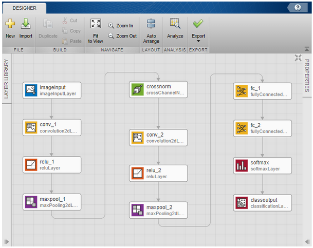
Figure 4: Deep Network Designer App in MATLAB
Once you have the tested your algorithm on your test image dataset, you can connect to your Jetson board from MATLAB to prototype your algorithm directly on the Jetson board. For this example, we chose the Jetson Nano board and as you can see in Figure 7, once you connect to the board using an addon support package, it also checks to make sure all the necessary software packages are installed. You can now test your algorithm on images captured from the webcam connected to the Jetson Nano by simply invoking the snapshot method of the webcam object in MATLAB as shown below:
>> hwobj=jetson(‘Device_address’,’username’,’password’);
Checking for CUDA availability on the Target…
Checking for ‘nvcc’ in the target system path…
Checking for cuDNN library availability on the Target…
Checking for TensorRT library availability on the Target…
Checking for prerequisite libraries is complete.
Gathering hardware details…
Gathering hardware details is complete.
Board name : NVIDIA Jetson TX1
CUDA Version : 10.0
cuDNN Version : 7.3
TensorRT Version : 5.0
Available Webcams :
Available GPUs : NVIDIA Tegra X1
>> img=hwobj.webcam.snapshot;
>>
Once we have read the image input from the camera connected to the Jetson Nano, we tested our application in MATLAB. In this example, we had to tweak the number of connected pixels parameter for the bwareaopen function to calibrate for the image from the camera. This is a typical use case for validating the robustness of your algorithm and flush out any issues before generating code and deploying your application because often your sensor input data may not be exactly the same as your training and test data.
Next, we generate CUDA code from our application and as explained in detail in the webinar, you can generate optimized CUDA source code or a static library or an executable by configuring the code generation configuration object. Figure 8 shows the configuration object we used to generate a static library targeting the Jetson Nano. The codegen command uses the configuration object to generate optimized CUDA code and then compiles it into a static library using the nvcc compiler on the Jetson board. We have also enabled the PIL verification mode and the CodeExecutionProfiling option to true. This will enable us to pass the data to and from the application on the hardware to MATLAB. We will discuss this in detail in the next section.
cfg = coder.gpuConfig(‘lib’);
cfg.DeepLearningConfig = coder.DeepLearningConfig(‘tensorrt’);
cfg.Hardware = coder.hardware(‘NVIDIA Jetson’);
cfg.VerificationMode=’PIL’;
cfg.CodeExecutionProfiling = true;
cfg.Hardware.DeviceAddress=’jetson-nano’;
cfg.Hardware.Username=’username’;
cfg.Hardware.Password=’password’;
codegen(‘-config’,cfg,’targetFunction’,’-args’,{img_test},’-report’);
Once the code generation is complete, you can generate the code traceability report as shown in Figure 9 below to understand the generated code by mapping it to the MATLAB code. The generated code leverages the compute power of the GPU to accelerate not only the deep learning inference, but the entire application including pre- and post-processing logic. Figure 5 highlights the section of the CUDA code on the right that corresponds to the predict function in MATLAB on the right and you can see the corresponding kernel calls and the cudaMemcpy calls.
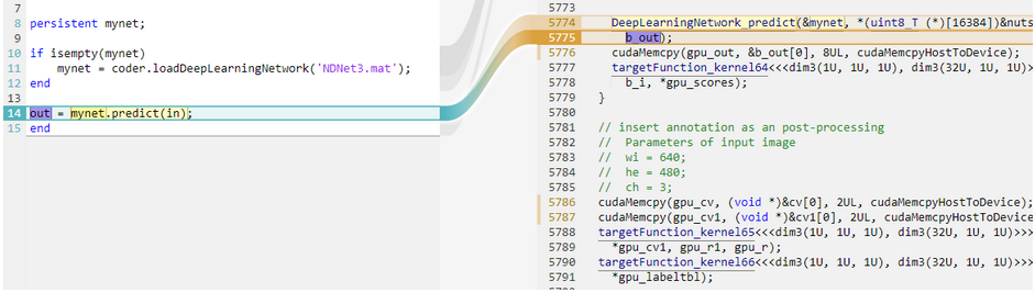
Figure 5: Code generation report to trace the generated CUDA kernels to the corresponding MATLAB code
Next, we are going to verify the equivalence of the algorithm and the generated code, through hardware-in-the-loop simulation. Hardware-in-the-loop simulation is a common approach to test the generated code on the hardware in the context of a bigger application being simulated in MATLAB. The hardware support package APIs enable you to run the executable on the Jetson Nano and to communicate back and forth with MATLAB. You can then use the test data in MATLAB as input and compare the output of the executable against the expected output in MATLAB. This allows you to compare not only the equivalence of the algorithm, but the instrumentation hooks in the executable also enables you to get a measure of the runtime performance of your application. We ran inference on about 150 test images using PIL, and we observed about 18 fps inference speed on the Jetson Nano. This is not an exact measure of the run-time performance on the Jetson because of the additional overhead of the instrumentation, to collect the profiling data, but gives you a good estimate of the expected run-time performance.
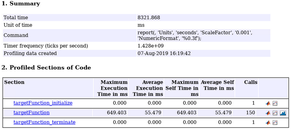
Figure 6: Code execution profile for our application from Jetson Nano
In fact, we ran a quick test to compare the performance of our application between the Jetson Xavier and Jetson Nano. This can be done very easily by simply changing the argument to the Jetson API to connect to the right Jetson board. We then used similar API to generate C++ code to run on the Raspberry Pi and you can see the comparison in Figure 7.
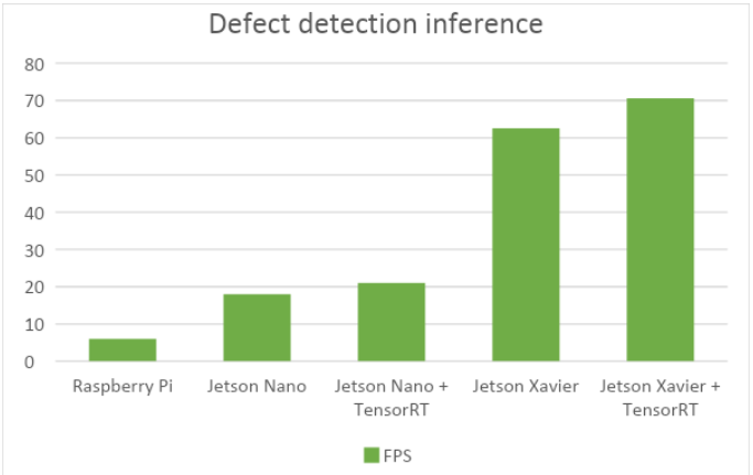
Figure 7: Comparison of the inference speed based on the PIL execution profile.
Finally, we can deploy our algorithm as a standalone application by simply updating the code generation configuration.
cfg = coder.gpuConfig(‘exe’);
In addition, we also updated our application to read the input directly from the webcam and to display the output image on the output display connected to the Jetson. The support package generates the necessary code to interface with the camera connected to the Jetson Nano avoiding the need for manual coding or integration enabling engineers to go from algorithm development to rapid prototyping to deployment in a seamless workflow.
hwobj = jetson;
w = webcam(hwobj);
d = imageDisplay(hwobj);
Conclusion
In this blog, we shared how you can prototype and deploy your deep learning algorithms on NVIDIA Jetson platforms from MATLAB. The workflow greatly simplifies the design iterations and debugging when going from development to deployment on the hardware. If you are interested in further exploring the NVIDIA hardware support package, check out the additional resources below.
Additional Resources:
Ram Cherukuri
Product Manager, MathWorks